Are Air Showers all the Same?
By Max Walent, May 8, 2019
Article: “Universality of Electron Distributions in Extensive Air Showers”
Authors: A. Smialkowski & M. Giller
Reference: arXiv:1801.00619 [astro-ph.HE]
So today’s paper focuses on air showers, the fallout of a high energy cosmic ray hitting the Earth’s atmosphere. Before we dive into the main paper, first I will begin with …
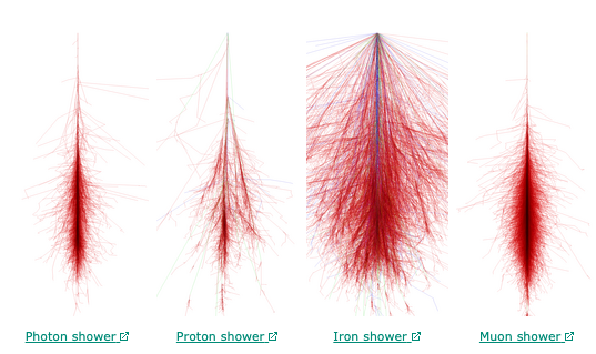
Figure 1: Simulated image from CORSIKA webpage, showing different sorts of air showers depending on the primary. Compiled by Fabian Schmidt, University of Leeds, UK. In all images the shower axis is pointing down, distance from this axis is the horizontal distance from the central line, the depth is the distance along the axis, the azimuthal angle is the angle between a resulting air shower particle’s motion and the shower axis, and the polar angle is the direction of motion around the axis.
A quick background on air showers:
Particles from outer space travel to Earth and impact with the atmosphere. The impacting particles are called primary particles (or primaries). These primaries interact with matter in the atmosphere and create more particles (see Figure 1 to the right). If the primaries have sufficient energy (~1017 eV) they will produce a particle shower. This occurs when the primary particle impacts with another particle in the atmosphere, resulting in the creation of new particles, and these new particles then impact again basically creating an avalanche. The vast majority of the created particles will decay within the atmosphere, while a small number will travel to the surface of the Earth. These showers are detected through the use of telescope arrays that see the light they emit, either visible or non-visible. Through the detection of this light (generated from the secondary particles) the properties of the primary particle are reconstructed, allowing us to understand more about the primaries.
Understanding these primary particles is useful for particle astrophysics in that it allows us to look at particles with a large range of energies, including many with energies well above what can be recreated on Earth with collider experiments, such as the LHC. These primary particles will also contain information on their origin, so we might puzzle out how they were created and where they came from. This is one of the techniques employed in the search for dark matter, or more specifically the indirect detection of dark matter.
The Paper:
This paper seeks to show that the initial conditions of the primary do not influence the electron distribution (fraction of electrons that have a certain energy that are travelling in a particular direction at a scaled distance from its creation) created by that primary, provided the electron distributions are properly compared (more on this later). Specifically, the conditions of the primary’s energy, mass, zenith angle, or other characteristics do not influence the electron distribution. While the previous work of these authors focused on electron distributions for fixed electron energies and varying lateral distance and angles, this is the first work to vary all the electron variables, including the directional angle, together.
This paper focuses on factors depending on the age of the shower, where the age of the shower, s, refers to the distance the shower has started from its inception. This is calculated by s(X) = 3X / (X + 2Xmax), for a given atmospheric depth, X. The age varies from 0 at the beginning of the shower, to beyond 1, where s = 1 occurs at the depth of maximum energy deposit, Xmax.
The equation of electron states is: ΔN(θ,φ,r/rM,E;s) = N(s) f(θ,φ,r/rM,E;s) Δθ Δφ Δlog(r/rM) ΔlogE, which honestly looks terrifying. Let’s step through it piece by piece. First N(s) is the total number of electrons that have an age s. f(θ,φ,r/rM,E;s), or f(x) for short, is the electron distribution, giving the fraction of electrons that would be found within some small energy range ΔlogE around E (it’s in logarithmic space because of the huge range in energies that are considered), and within some small range in distance from the shower axis (see Figure 1 above) Δlog(r/rM) around a given distant r/rM (it is common to rescale this distance by the Molière radius, rM so that the units are sensible), within some small angular range Δφ around an azimuthal angle φ, and within some small angular range Δθ around a polar angle θ. So ΔN(θ,φ,r/rM,E;s) is the total number of electrons of a given age s in an air shower that have a particular set of characteristics. This paper demonstrates that for consideration of large numbers of electrons within any given bin (ΔN > 100), the functional form of f(x) is universal, regardless of the characteristics of the primary, provided you scale to the same shower age, s. Note that the shower age is dependent on the primary characteristics.
The distribution equation f(x) can be further broken down into a product of distributions for each variable, f(θ,φ,r/rM,E;s) = fE(E;s) fr(r/rM;E,s) fφ(φ;r/rM,E,s) fθ(θ;φ,r/rM,E,s). Whereas past papers looked at the dependence of f(x) on electron energy, this paper focuses on its dependence on the distributions fθ and fφ.
The authors use simulation data of air showers generated with the specialized programs CORSIKA (see Figure 1 above) and QGSJET–II. The simulations considered various variable ranges, in particular a primary energy of 1016 eV – 1019 eV. The results for the determination of fφ can be seen in Figures 2 below.
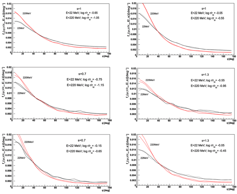
Figure 2: Taken from Figures 1 (top) and 2 (middle and bottom) from the paper, showing fφ for different electron energies (red vs black) and primary energies (solid vs dotted). Universality is roughly shown, as different primary energies do not change the general functional form of fφ. The authors note that for an age of s = 1 universality is the clearest.
This figure shows the fφ distributions over φ for various electron energies, distances from the shower axis, and shower ages. They do this for two different primary energies (1 proton primary with energy 1019 eV in solid, and an average of 10 iron primaries each with energy 1017 eV in the dotted lines). The different primary energies do not show much difference in the distribution, consistent with universality.
The results for fθ are then explored by the authors, which are shown below in Figure 3. Similar to Figure 2, the fθ distributions over θ for various electron energies and distances from the shower axis (all plots have a shower age of 1, as other ages give very similar results). They do this for two different primary energies (1 proton primary with energy 1019 eV in solid, and an average of 10 iron primaries each with energy 1016 eV in the dotted lines, with a single iron primary shown with the histogram). Universality is even clearer here.
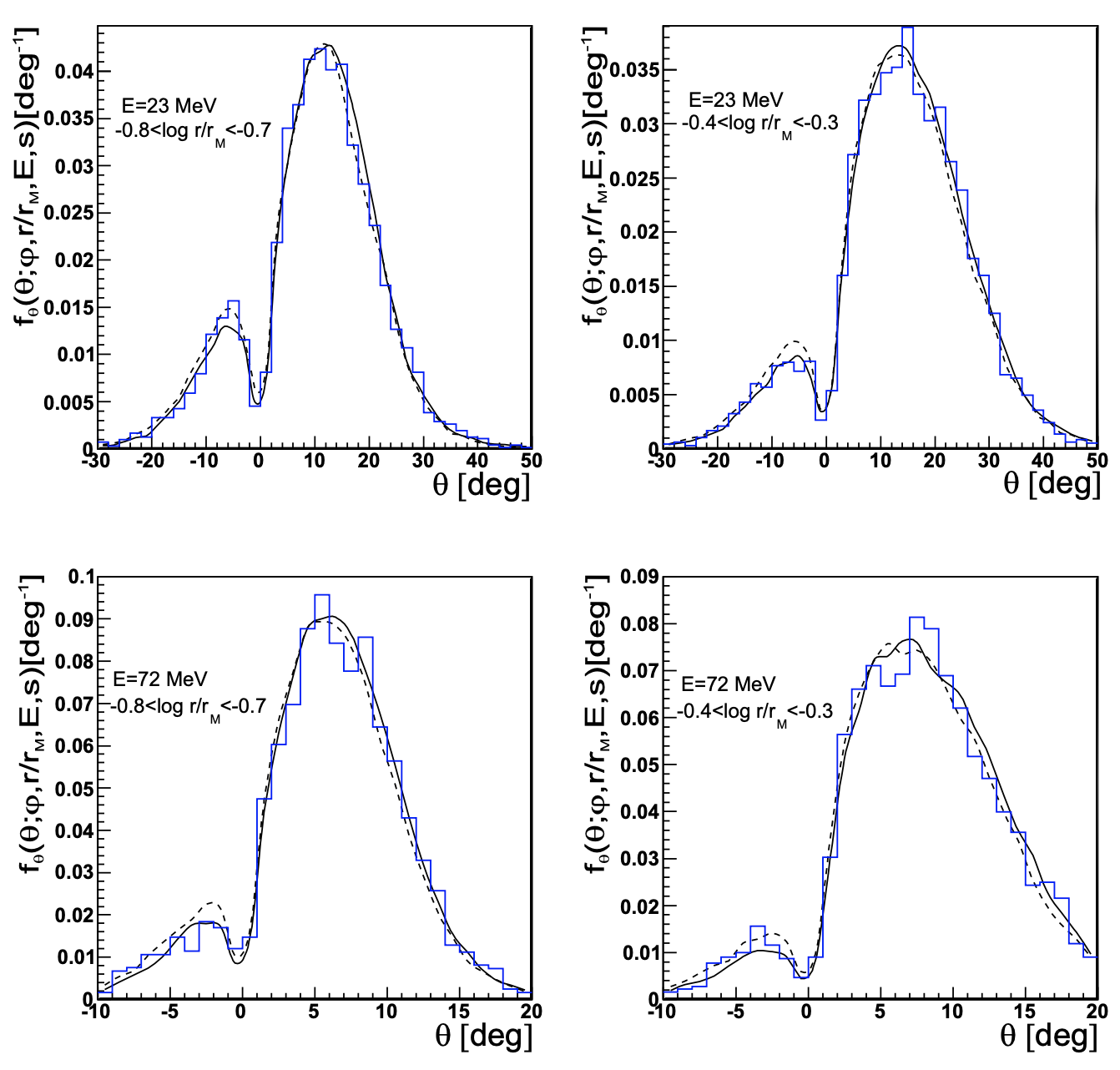
Figure 3 from the paper showing fθ for different electron energy, radius, and azimuthal angle, all with an age of 1 (the results are similar for other ages). Again, different line styles are for different primary energy, showing the strong universality discussed in the paper.
Given the demonstrated independence of the two angular distribution functions on the primary characteristics, the rest of the paper determines universal functions for these two distributions in terms of the electron energy and radius. The authors find that fφ has a specific dependence on energy and radius, simplifying it to a dependence on χ = (E/MeV)(r/rM). Likewise, a transformation of θ gives a universal function for fθ, with ξ = (E/GeV)α(1 + r/rM)θ/(r/rM)β, where α and β are best fit parameters that depend on φ. With these transformation, the distributions simplify significant, which is shown in the figure below.
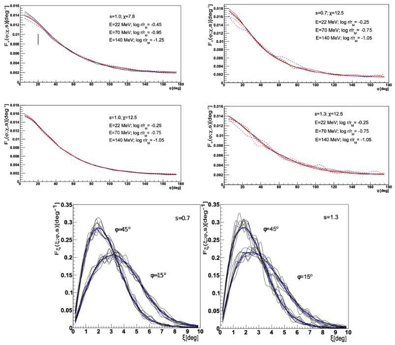
Figures 5 (top), 6 (middle), and 7 (bottom) from the text. All plots are for distributions dependent on χ and ξ rather than the energy, distance, and azimuthal angle independently. For Fφ this resulted in an almost direct matching of the electron azimuthal angle distribution across different electron energies and distances. For the bottom panels, the thick blue line is average distributions for all energies, distances, and θ angles for a proton shower of the energy 1019 eV. Individual values of the parameters correspond to different thin black lines, which do lead to perturbations in the distribution.
The resulting distribution functions show clear universality in φ, however the θ distribution has large fluctuations around the universal model. The paper suggests this can be improved by accounting for the Earth’s geomagnetic field.
There are a number of things to consider when interpreting these results.
- The simulations were done with the initial energy (and other conditions) of the primary that were “somewhat arbitrarily chosen”. Further study should explore a larger range of primary energies
- The results from these conditions were taken as an average. The results of a single (measured) shower can diverge from the average.
- The functions used to fit the variables may be too simple to cover all regions of the variables.
- There were difficulties in determining the shower age of the simulated shower. This results in derived electron distributions diverging from chosen ones.
- The initial conditions of the primary may be outside the range of initial conditions chosen for the primary in this paper.
What follows in the paper is calculations of errors, and the determination that these results are suggestive. There is also a correction calculated that needs to be added to the electron distribution due to the geomagnetic field (Earth’s magnetic field) as it was initially assumed to be zero.
In summary, this paper is the last part in a series of papers that gradually include more variables describing the electron state in an air shower. Initially, electron energy spectra were shown to be universal and only dependent upon shower age (Giller et al. 2004). Followed by the lateral distributions being shown to be universal (Giller et al. 2005b; Nerling et al. 2006). This work now shows that this extends to the angular distributions of electrons.
Angular distributions of electrons, dependent on the electron energy and lateral distance have been found. The number of variables used to describe these parameters has been reduced to below 5. For primaries within the energy range 1016 eV – 1019 eV.
The results in this paper allow for better reconstruction of primaries using florescence techniques. This is through the prediction of the light flux emitted by the electron distribution. This method is particularly useful for showers with a small angle between the shower axis and the camera symmetry axis. This is because these types of showers produce a significant amount of Cherenkov light. If employing this technique one should consider some of the possible inaccuracies listed previously. Nevertheless, this work points towards a simple but powerful technique to better understand the nature of primaries of air shower, which is important for probing the high energy particle physics regime.


About Max Walent
I’m a first year masters student at Laurentian University, currently working on reducing the Rn backgrounds from the nEXO plumbing system.